ML_R Kmeans
Kmeans作为机器学习中入门级算法,涉及到计算距离算法的选择,聚类中心个数的选择。下面就简单介绍一下在R语言中是怎么解决这两个问题的。
参考Unsupervised Learning with R
> Iris<-iris

> #K mean

> set.seed(123)

> KM.Iris<-kmeans(Iris[1:4],3,iter.max=1000,algorithm = c("Forgy"))

> KM.Iris$size

[1] 50 39 61

> KM.Iris$centers  #聚类的3个中心

  Sepal.Length Sepal.Width Petal.Length Petal.Width

1     5.006000    3.428000     1.462000    0.246000

2     6.853846    3.076923     5.715385    2.053846

3     5.883607    2.740984     4.388525    1.434426

> str(KM.Iris)

List of 9

 $ cluster     : int [1:150] 1 1 1 1 1 1 1 1 1 1 ...

 $ centers     : num [1:3, 1:4] 5.01 6.85 5.88 3.43 3.08 ...

  ..- attr(*, "dimnames")=List of 2

  .. ..$ : chr [1:3] "1" "2" "3"

  .. ..$ : chr [1:4] "Sepal.Length" "Sepal.Width" "Petal.Length" "Petal.Width"

 $ totss       : num 681

 $ withinss    : num [1:3] 15.2 25.4 38.3

 $ tot.withinss: num 78.9

 $ betweenss   : num 603

 $ size        : int [1:3] 50 39 61

 $ iter        : int 2

 $ ifault      : NULL

 - attr(*, "class")= chr "kmeans"
> table(Iris$Species,KM.Iris$cluster)
1 2 3
setosa 50 0 0
versicolor 0 3 47
virginica 0 36 14
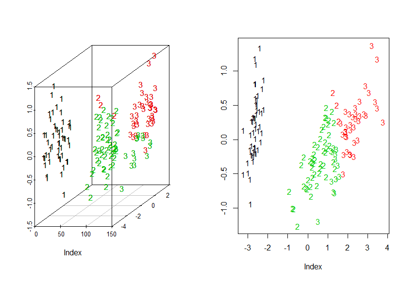
> Iris.dist<-dist(Iris[1:4])
> Iris.mds<-cmdscale(Iris.dist)
关于cmdscale,classical multidimensional scaling of a data matrix,也被成为是principal coordinates analysis
> par(mfrow=c(1,2))

> #3D

> library("scatterplot3d")

> chars<-c("1","2","3")[as.integer(iris$Species)]

> g3d<-scatterplot3d(Iris.mds,pch=chars)

> g3d$points3d(iris.mds,col=KM.Iris$cluster,pch=chars)

> #2D

> plot(Iris.mds,col=KM.Iris$cluster,pch=chars,xlab="Index",ylab= "Y")
> KM.Iris[1]
$cluster
[1] 1 1 1 1 1 1 1 1 1 1 1 1 1 1 1 1 1 1 1 1 1 1 1 1 1 1 1 1 1 1 1 1 1 1 1 1 1 1 1 1 1 1 1 1 1 1 1 1 1 1 2 3 2 3 3 3 3 3
[59] 3 3 3 3 3 3 3 3 3 3 3 3 3 3 3 3 3 3 3 2 3 3 3 3 3 3 3 3 3 3 3 3 3 3 3 3 3 3 3 3 3 3 2 3 2 2 2 2 3 2 2 2 2 2 2 3 3 2
[117] 2 2 2 3 2 3 2 3 2 2 3 3 2 2 2 2 2 3 2 2 2 2 3 2 2 2 3 2 2 2 3 2 2 3
> Iris.cluster<-cbind(Iris,KM.Iris$cluster)
> head(Iris.cluster)
Sepal.Length Sepal.Width Petal.Length Petal.Width Species KM.Iris$cluster
1 5.1 3.5 1.4 0.2 setosa 1
2 4.9 3.0 1.4 0.2 setosa 1
3 4.7 3.2 1.3 0.2 setosa 1
4 4.6 3.1 1.5 0.2 setosa 1
5 5.0 3.6 1.4 0.2 setosa 1
6 5.4 3.9 1.7 0.4 setosa 1
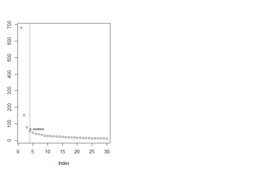
> # 下面寻找最佳簇数目
> # 30 Kmeans loop
> InerIC<-rep(0,30);InerIC
[1] 0 0 0 0 0 0 0 0 0 0 0 0 0 0 0 0 0 0 0 0 0 0 0 0 0 0 0 0 0 0
> for (k in 1:30){
+ set.seed(123)
+ groups=kmeans(Iris[1:4],k)
+ InerIC[k]<-groups$tot.withinss
+ }
> InerIC
[1] 681.37060 152.34795 78.85144 57.26562 46.46117 39.05498 37.34900 32.58266 28.46897 26.32133 24.92591
[12] 23.52298 23.33464 21.83167 20.04231 19.21720 17.82750 17.35801 16.69589 15.74660 14.53898 13.61800
[23] 13.38004 12.81350 12.37310 12.02532 11.72245 11.55765 11.04824 10.56507
> groups
K-means clustering with 30 clusters of sizes 5, 4, 1, 5, 7, 5, 9, 3, 4, 2, 3, 4, 3, 7, 4, 5, 8, 5, 4, 3, 9, 1, 6, 4, 4, 8, 1, 3, 10, 13
Cluster means:
Sepal.Length Sepal.Width Petal.Length Petal.Width
1 4.940000 3.400000 1.680000 0.3800000
2 7.675000 2.850000 6.575000 2.1750000
3 5.000000 2.000000 3.500000 1.0000000
4 7.240000 2.980000 6.020000 1.8400000
5 6.442857 2.828571 5.557143 1.9142857
6 4.580000 3.320000 1.280000 0.2200000
7 6.722222 3.000000 4.677778 1.4555556
8 6.233333 3.300000 4.566667 1.5666667
9 6.150000 2.900000 4.200000 1.3500000
10 5.400000 2.800000 3.750000 1.3500000
11 6.133333 2.700000 5.266667 1.5000000
12 6.075000 2.900000 4.625000 1.3750000
13 5.000000 2.400000 3.200000 1.0333333
14 6.671429 3.085714 5.257143 2.1571429
15 4.400000 2.800000 1.275000 0.2000000
16 5.740000 2.700000 5.040000 2.0400000
17 5.212500 3.812500 1.587500 0.2750000
18 5.620000 4.060000 1.420000 0.3000000
19 5.975000 3.050000 4.900000 1.8000000
20 7.600000 3.733333 6.400000 2.2333333
21 6.566667 3.244444 5.711111 2.3333333
22 4.900000 2.500000 4.500000 1.7000000
23 5.550000 2.450000 3.816667 1.1333333
24 6.275000 2.625000 4.900000 1.7500000
25 5.775000 2.700000 4.025000 1.1750000
26 5.600000 2.875000 4.325000 1.3250000
27 6.000000 2.200000 4.000000 1.0000000
28 6.166667 2.233333 4.633333 1.4333333
29 4.840000 3.080000 1.470000 0.1900000
30 5.146154 3.461538 1.438462 0.2230769
Clustering vector:
[1] 30 29 6 29 30 17 6 30 15 29 17 1 29 15 18 18 18 30 18 17 30 17 6 1 1 29 1 30 30 29 29 30 17 18 29 29 30 30 15
[40] 30 30 15 6 1 17 29 17 6 17 30 7 8 7 23 7 26 8 13 7 10 3 9 27 12 10 7 26 25 28 23 19 9 24 12 9 7 7 7
[79] 12 23 23 23 25 11 26 8 7 28 26 23 26 12 25 13 26 26 26 9 13 25 21 16 4 5 21 2 22 4 5 20 14 5 14 16 16 14 5
[118] 20 2 28 21 16 2 24 21 4 24 19 5 4 4 20 5 11 11 2 21 5 19 14 21 14 16 21 21 14 24 14 21 19
Within cluster sum of squares by cluster:
[1] 0.2880000 0.5325000 0.0000000 0.4200000 0.6371429 0.2920000 0.7933333 0.1400000 0.2400000 0.1500000 0.2533333
[12] 0.1025000 0.1066667 0.5571429 0.4275000 0.2960000 0.5012500 0.5280000 0.1175000 0.5933333 1.0311111 0.0000000
[23] 0.3716667 0.1850000 0.1025000 0.5450000 0.0000000 0.2866667 0.3700000 0.6969231
(between_SS / total_SS = 98.4 %)
Available components:
[1] "cluster" "centers" "totss" "withinss" "tot.withinss" "betweenss" "size"
[8] "iter" "ifault"
> plot(InerIC,col = "black",lty =3)
There were 18 warnings (use warnings() to see them)
> abline(v=4,col="black",lty=3)
> text (4,60,"4 clusters",col="black",adj = c(0,-0.1),cex=0.7)
> library(NbClust)

> data<-Iris[,-5]

> head(data)

  Sepal.Length Sepal.Width Petal.Length Petal.Width

1          5.1         3.5          1.4         0.2

2          4.9         3.0          1.4         0.2

3          4.7         3.2          1.3         0.2

4          4.6         3.1          1.5         0.2

5          5.0         3.6          1.4         0.2

6          5.4         3.9          1.7         0.4

> best<-NbClust(data,diss=NULL,distance ="euclidean",min.nc=2, max.nc=15, method = "complete",index = "alllong")

*** : The Hubert index is a graphical method of determining the number of clusters.

                In the plot of Hubert index, we seek a significant knee that corresponds to a

                significant increase of the value of the measure i.e the significant peak in Hubert

                index second differences plot.
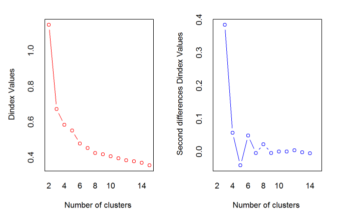
*** : The D index is a graphical method of determining the number of clusters.
In the plot of D index, we seek a significant knee (the significant peak in Dindex
second differences plot) that corresponds to a significant increase of the value of
the measure.
*******************************************************************
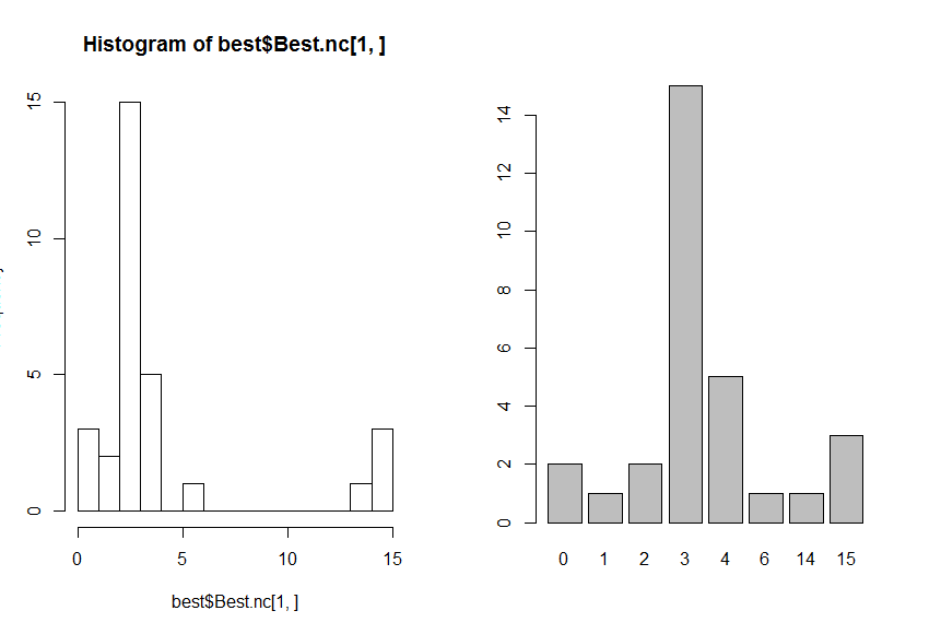
* Among all indices:
* 2 proposed 2 as the best number of clusters
* 15 proposed 3 as the best number of clusters
* 5 proposed 4 as the best number of clusters
* 1 proposed 6 as the best number of clusters
* 1 proposed 14 as the best number of clusters
* 3 proposed 15 as the best number of clusters
***** Conclusion *****
* According to the majority rule, the best number of clusters is 3
*******************************************************************
> table(names(best$Best.nc[1,]),best$Best.nc[1,])
0 1 2 3 4 6 14 15
Ball 0 0 0 1 0 0 0 0
Beale 0 0 0 1 0 0 0 0
CCC 0 0 0 1 0 0 0 0
CH 0 0 0 0 1 0 0 0
Cindex 0 0 0 1 0 0 0 0
DB 0 0 0 1 0 0 0 0
Dindex 1 0 0 0 0 0 0 0
Duda 0 0 0 0 1 0 0 0
Dunn 0 0 0 0 0 0 0 1
Frey 0 1 0 0 0 0 0 0
Friedman 0 0 0 0 1 0 0 0
Gamma 0 0 0 0 0 0 1 0
Gap 0 0 0 1 0 0 0 0
Gplus 0 0 0 0 0 0 0 1
Hartigan 0 0 0 1 0 0 0 0
Hubert 1 0 0 0 0 0 0 0
KL 0 0 0 0 1 0 0 0
Marriot 0 0 0 1 0 0 0 0
McClain 0 0 1 0 0 0 0 0
PseudoT2 0 0 0 0 1 0 0 0
PtBiserial 0 0 0 1 0 0 0 0
Ratkowsky 0 0 0 1 0 0 0 0
Rubin 0 0 0 0 0 1 0 0
Scott 0 0 0 1 0 0 0 0
SDbw 0 0 0 0 0 0 0 1
SDindex 0 0 0 1 0 0 0 0
Silhouette 0 0 1 0 0 0 0 0
Tau 0 0 0 1 0 0 0 0
TraceW 0 0 0 1 0 0 0 0
TrCovW 0 0 0 1 0 0 0 0
> hist(best$Best.nc[1,],breaks = max(na.omit(best$Best.nc[1,])))
> barplot(table(best$Best.nc[1,]))
> # 选择最佳聚类算法algorithm
> Hartigan <-0
> Lloyd <- 0
> Forgy <- 0
> MacQueen <- 0
> set.seed(123)
> # 做500次Kmeans计算,3个聚类中心,每次计算,每种算法迭代最多1000次
> for (i in 1:500){
+ KM<-kmeans(Iris[1:4],3,iter.max = 1000,algorithm = "Hartigan-Wong")
+ Hartigan <- Hartigan + KM$betweenss
+ KM<-kmeans(Iris[1:4],3,iter.max = 1000,algorithm = "Lloyd")
+ Lloyd <- Lloyd + KM$betweenss
+ KM<-kmeans(Iris[1:4],3,iter.max = 1000,algorithm = "Forgy")
+ Forgy <- Forgy + KM$betweenss
+ KM<-kmeans(Iris[1:4],3,iter.max = 1000,algorithm = "MacQueen")
+ MacQueen <- MacQueen + KM$betweenss
+ }
> # 输出结果
> Methods <- c("Hartigan","Lloyd","Forgy","MacQueen")
> Results <- as.data.frame(round(c(Hartigan,Lloyd,Forgy,MacQueen)/500,2))
> Results <- cbind(Methods,Results)
> names(Results) <- c("Method","Betweenss")
> Results
Method Betweenss
1 Hartigan 590.76
2 Lloyd 589.38
3 Forgy 590.63
4 MacQueen 590.05
> #作图
> par(mfrow =c(1,1))
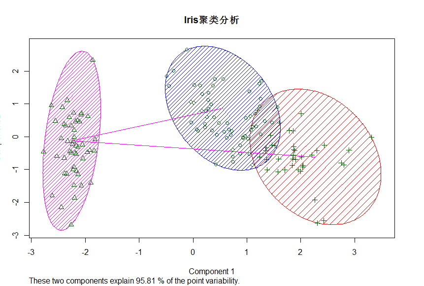
> KM<-kmeans(Iris[1:4],3,iter.max = 1000,algorithm = "Hartigan-Wong")
> library(cluster)
> clusplot(Iris[1:4],KM$cluster,color = T,shade = T,lables=2,lines = 1,main = "Iris聚类分析")
There were 50 or more warnings (use warnings() to see the first 50)
> library(HSAUR)
There were 50 or more warnings (use warnings() to see the first 50)
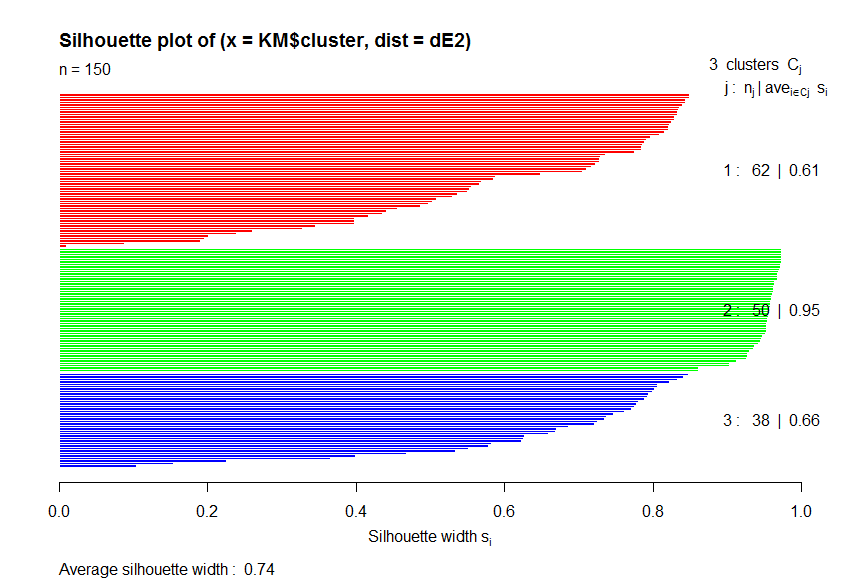
> diss <- daisy(Iris[1:4])
> dE2 <- diss^2
> obj <-silhouette(KM$cluster,dE2)
> plot(obj,col=c("red","green","blue"))
ML_R Kmeans的更多相关文章
- 当我们在谈论kmeans(1)
本稿为初稿,后续可能还会修改:如果转载,请务必保留源地址,非常感谢! 博客园:http://www.cnblogs.com/data-miner/ 简书:建设中... 知乎:建设中... 当我们在谈论 ...
- K-Means 聚类算法
K-Means 概念定义: K-Means 是一种基于距离的排他的聚类划分方法. 上面的 K-Means 描述中包含了几个概念: 聚类(Clustering):K-Means 是一种聚类分析(Clus ...
- 用scikit-learn学习K-Means聚类
在K-Means聚类算法原理中,我们对K-Means的原理做了总结,本文我们就来讨论用scikit-learn来学习K-Means聚类.重点讲述如何选择合适的k值. 1. K-Means类概述 在sc ...
- K-Means聚类算法原理
K-Means算法是无监督的聚类算法,它实现起来比较简单,聚类效果也不错,因此应用很广泛.K-Means算法有大量的变体,本文就从最传统的K-Means算法讲起,在其基础上讲述K-Means的优化变体 ...
- kmeans算法并行化的mpi程序
用c语言写了kmeans算法的串行程序,再用mpi来写并行版的,貌似参照着串行版来写并行版,效果不是很赏心悦目~ 并行化思路: 使用主从模式.由一个节点充当主节点负责数据的划分与分配,其他节点完成本地 ...
- 当我们在谈论kmeans(2)
本稿为初稿,后续可能还会修改:如果转载,请务必保留源地址,非常感谢! 博客园:http://www.cnblogs.com/data-miner/ 其他:建设中- 当我们在谈论kmeans(2 ...
- K-Means clusternig example with Python and Scikit-learn(推荐)
https://www.pythonprogramming.net/flat-clustering-machine-learning-python-scikit-learn/ Unsupervised ...
- K-Means聚类和EM算法复习总结
摘要: 1.算法概述 2.算法推导 3.算法特性及优缺点 4.注意事项 5.实现和具体例子 6.适用场合 内容: 1.算法概述 k-means算法是一种得到最广泛使用的聚类算法. 它是将各个聚类子集内 ...
- 【原创】数据挖掘案例——ReliefF和K-means算法的医学应用
数据挖掘方法的提出,让人们有能力最终认识数据的真正价值,即蕴藏在数据中的信息和知识.数据挖掘 (DataMiriing),指的是从大型数据库或数据仓库中提取人们感兴趣的知识,这些知识是隐含的.事先未知 ...
随机推荐
- Linux下修改进程名称
catalog . 应用场景 . 通过Linux prctl修改进程名 . 通过修改进程argv[]修改进程名 . 通过bash exec命令修改一个进程的cmdline信息 1. 应用场景 . 标识 ...
- dedecms /include/uploadsafe.inc.php SQL Injection Via Local Variable Overriding Vul
catalog . 漏洞描述 . 漏洞触发条件 . 漏洞影响范围 . 漏洞代码分析 . 防御方法 . 攻防思考 1. 漏洞描述 . dedecms原生提供一个"本地变量注册"的模拟 ...
- Scala Trait
Scala Trait 大多数的时候,Scala中的trait有点类似于Java中的interface.正如同java中的class可以implement多个interface,scala中的cals ...
- Scala高阶函数示例
object Closure { def function1(n: Int): Int = { val multiplier = (i: Int, m: Int) => i * m multip ...
- CF 468A 24 Game
题目链接: 传送门 24 Game time limit per test:1 second memory limit per test:256 megabytes Description L ...
- Java反射机制实例解析
1.获取想操作的访问类的java.lang.Class类的对象 2.调用Class对象的方法返回访问类的方法和属性信息 3.使用反射API来操作 每个类被加载后,系统会为该类 ...
- Appium for IOS testing on Mac
一:环境 1.Mac OS X 10.9.1 2.Xcod 5.0.2 3.Appium 1.3.6 下载地址:https://bitbucket.org/appium/appium.app/down ...
- linux学习笔记-dump命令的使用
http://blog.chinaunix.net/uid-29797586-id-4458302.html
- windows系统下安装MySQL
可以运行在本地windows版本的MySQL数据库程 序自从3.21版以后已经可以从MySQL AB公司获得,而且 MYSQL每日的下载百分比非常大.这部分描述在windows上安装MySQL的过程. ...
- spark 加载文件
spark 加载文件 textFile的参数是一个path,这个path可以是: 1. 一个文件路径,这时候只装载指定的文件 2. 一个目录路径,这时候只装载指定目录下面的所有文件(不包括子目录下面的 ...