Andrew Ng机器学习 四：Neural Networks Learning

　　

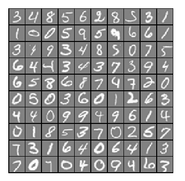
　　背景：跟上一讲一样，识别手写数字，给一组数据集ex4data1.mat，，每个样例都为灰度化为20*20像素，也就是每个样例的维度为400，加载这组数据后，我们会有5000*400的矩阵X(5000个样例)，5000*1的矩阵y(表示每个样例所代表的数据)。现在让你拟合出一个模型，使得这个模型能很好的预测其它手写的数字。

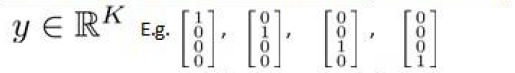
（注意：我们用10代表0(矩阵y也是这样)，因为Octave的矩阵没有0行）

一：神经网络( Neural Networks)

　　神经网络脚本ex4.m：

%% Machine Learning Online Class - Exercise  Neural Network Learning

%  Instructions
%  ------------
%
%  This file contains code that helps you get started on the
%  linear exercise. You will need to complete the following functions
%  in this exericse:
%
%     sigmoidGradient.m
%     randInitializeWeights.m
%     nnCostFunction.m
%
%  For this exercise, you will not need to change any code in this file,
%  or any other files other than those mentioned above.
%

%% Initialization
clear ; close all; clc

%% Setup the parameters you will use for this exercise
input_layer_size  = ;  % 20x20 Input Images of Digits
hidden_layer_size = ;   %  hidden units
num_labels = ;          %  labels, from  to
                          % (note that we have mapped "" to label )

%% =========== Part : Loading and Visualizing Data =============
%  We start the exercise by first loading and visualizing the dataset.
%  You will be working with a dataset that contains handwritten digits.
%

% Load Training Data
fprintf('Loading and Visualizing Data ...\n')

load('ex4data1.mat');
m = size(X, );

% Randomly select  data points to display
sel = randperm(size(X, ));
sel = sel(:);

displayData(X(sel, :));

fprintf('Program paused. Press enter to continue.\n');
pause;

%% ================ Part : Loading Parameters ================
% In this part of the exercise, we load some pre-initialized
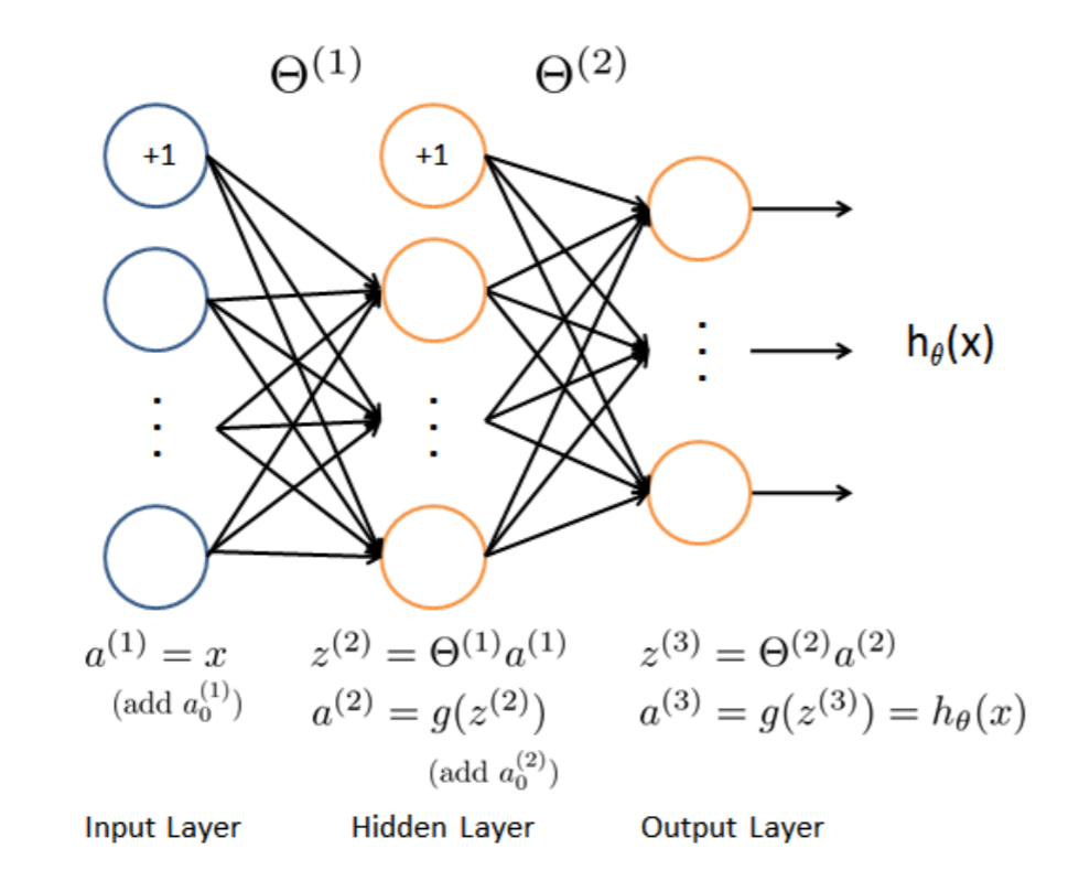
% neural network parameters.

fprintf('\nLoading Saved Neural Network Parameters ...\n')

% Load the weights into variables Theta1(25x401) and Theta2(10x26)
load('ex4weights.mat');

% Unroll parameters
nn_params = [Theta1(:) ; Theta2(:)];

%% ================ Part : Compute Cost (Feedforward) ================
%  To the neural network, you should first start by implementing the
%  feedforward part of the neural network that returns the cost only. You
%  should complete the code in nnCostFunction.m to return cost. After
%  implementing the feedforward to compute the cost, you can verify that
%  your implementation is correct by verifying that you get the same cost
%  as us for the fixed debugging parameters.
%
%  We suggest implementing the feedforward cost *without* regularization
%  first so that it will be easier for you to debug. Later, in part , you
%  will get to implement the regularized cost.
%
fprintf('\nFeedforward Using Neural Network ...\n')

% Weight regularization parameter (we set this to  here).
lambda = ;

J = nnCostFunction(nn_params, input_layer_size, hidden_layer_size, ...
                   num_labels, X, y, lambda);

fprintf(['Cost at parameters (loaded from ex4weights): %f '...
         '\n(this value should be about 0.287629)\n'], J);

fprintf('\nProgram paused. Press enter to continue.\n');
pause;

%% =============== Part : Implement Regularization ===============
%  Once your cost function implementation is correct, you should now
%  continue to implement the regularization with the cost.
%

fprintf('\nChecking Cost Function (w/ Regularization) ... \n')

% Weight regularization parameter (we set this to  here).
lambda = ;

J = nnCostFunction(nn_params, input_layer_size, hidden_layer_size, ...
                   num_labels, X, y, lambda);

fprintf(['Cost at parameters (loaded from ex4weights): %f '...
         '\n(this value should be about 0.383770)\n'], J);

fprintf('Program paused. Press enter to continue.\n');
pause;

%% ================ Part : Sigmoid Gradient  ================
%  Before you start implementing the neural network, you will first
%  implement the gradient for the sigmoid function. You should complete the
%  code in the sigmoidGradient.m file.
%

fprintf('\nEvaluating sigmoid gradient...\n')

g = sigmoidGradient([- -0.5  0.5 ]);
fprintf('Sigmoid gradient evaluated at [-1 -0.5 0 0.5 1]:\n  ');
fprintf('%f ', g);
fprintf('\n\n');

fprintf('Program paused. Press enter to continue.\n');
pause;

%% ================ Part : Initializing Pameters ================
%  In this part of the exercise, you will be starting to implment a two
%  layer neural network that classifies digits. You will start by
%  implementing a function to initialize the weights of the neural network
%  (randInitializeWeights.m)

fprintf('\nInitializing Neural Network Parameters ...\n')

initial_Theta1 = randInitializeWeights(input_layer_size, hidden_layer_size);
initial_Theta2 = randInitializeWeights(hidden_layer_size, num_labels);

% Unroll parameters
initial_nn_params = [initial_Theta1(:) ; initial_Theta2(:)];

%% =============== Part : Implement Backpropagation ===============
%  Once your cost matches up with ours, you should proceed to implement the
%  backpropagation algorithm for the neural network. You should add to the
%  code you've written in nnCostFunction.m to return the partial
%  derivatives of the parameters.
%
fprintf('\nChecking Backpropagation... \n');

%  Check gradients by running checkNNGradients
checkNNGradients;

fprintf('\nProgram paused. Press enter to continue.\n');
pause;

%% =============== Part : Implement Regularization ===============
%  Once your backpropagation implementation is correct, you should now
%  continue to implement the regularization with the cost and gradient.
%

fprintf('\nChecking Backpropagation (w/ Regularization) ... \n')

%  Check gradients by running checkNNGradients
lambda = ;
checkNNGradients(lambda);

% Also output the costFunction debugging values
debug_J  = nnCostFunction(nn_params, input_layer_size, ...
                          hidden_layer_size, num_labels, X, y, lambda);

fprintf(['\n\nCost at (fixed) debugging parameters (w/ lambda = %f): %f ' ...
         '\n(for lambda = 3, this value should be about 0.576051)\n\n'], lambda, debug_J);

fprintf('Program paused. Press enter to continue.\n');
pause;

%% =================== Part : Training NN ===================
%  You have now implemented all the code necessary to train a neural
%  network. To train your neural network, we will now use "fmincg", which
%  is a function which works similarly to "fminunc". Recall that these
%  advanced optimizers are able to train our cost functions efficiently as
%  long as we provide them with the gradient computations.
%
fprintf('\nTraining Neural Network... \n')

%  After you have completed the assignment, change the MaxIter to a larger
%  value to see how more training helps.
options = optimset('MaxIter', );

%  You should also try different values of lambda
lambda = ;

% Create "short hand" for the cost function to be minimized
costFunction = @(p) nnCostFunction(p, ...
                                   input_layer_size, ...
                                   hidden_layer_size, ...
                                   num_labels, X, y, lambda);

% Now, costFunction is a function that takes in only one argument (the
% neural network parameters)
[nn_params, cost] = fmincg(costFunction, initial_nn_params, options);

% Obtain Theta1 and Theta2 back from nn_params
Theta1 = reshape(nn_params(:hidden_layer_size * (input_layer_size + )), ...
                 hidden_layer_size, (input_layer_size + ));

Theta2 = reshape(nn_params(( + (hidden_layer_size * (input_layer_size + ))):end), ...
                 num_labels, (hidden_layer_size + ));

fprintf('Program paused. Press enter to continue.\n');
pause;

%% ================= Part : Visualize Weights =================
%  You can now "visualize" what the neural network is learning by
%  displaying the hidden units to see what features they are capturing in
%  the data.

fprintf('\nVisualizing Neural Network... \n')

displayData(Theta1(:, :end));

fprintf('\nProgram paused. Press enter to continue.\n');
pause;

%% ================= Part : Implement Predict =================
%  After training the neural network, we would like to use it to predict
%  the labels. You will now implement the "predict" function to use the
%  neural network to predict the labels of the training set. This lets
%  you compute the training set accuracy.

pred = predict(Theta1, Theta2, X);

fprintf('\nTraining Set Accuracy: %f\n', mean(double(pred == y)) * );

ex4.m

　　1，通过可视化数据，可以看到如下图所示：

　　2，前向传播代价函数(Feedforward and cost function)

　　

$J(\Theta)=-\frac{1}{m}\sum_{i=1}^{m}\sum_{k=1}^{K}[y^{(i)}_k(log(h_\Theta(x^{(i)}))_k)+(1-y^{(i)}_k)log(1-(h_{\Theta}(x^{(i)}))_k)]$

$+\frac{\lambda }{2m}\sum_{l=1}^{L-1}\sum_{i=1}^{s_l}\sum_{j=1}^{s_l+1}(\Theta_{ji}^{l})^{2}$

注意：$(h_\Theta(x^{(i)}))_k=a^{(3)}_k$，第k个输出单元。

该代价函数正则化时忽略偏差项，最里层的循环$