使用TensorBoard可视化工具

---

title: 使用TensorBoard可视化工具

date: 2018-04-01 13:04:00

categories:

• deep learning

tags:

• TensorFlow
• TensorBoard

---

图表可视化在理解和调试时显得非常有帮助。

安装：

pip3 install --upgrade tensorboard

名称域（Name scoping）和节点（Node）

典型的TensorFlow有数以千计的节点，为了简单起见，我们可以为变量名（节点）划分范围。

这个范围称为名称域，即tf.name_scope('xxx')，其中xxx是这个名称域的名字。

在定义好名称域后，TensorBoard的显示界面里这个名称域内的变量并不会显示，而是只显示一个xxx节点，这个点是可展开的，展开后才会显示这个名称域内的节点。

TensorFlow 图表有两种连接关系：数据依赖和控制依赖。数据依赖显示两个操作之间的tensor流程，用实心箭头表示，控制依赖用虚线表示。

具体的符号表：

符号	意义
	High-level节点代表一个名称域，双击则展开一个高层节点。
	彼此之间不连接的有限个节点序列。
	彼此之间相连的有限个节点序列。
	一个单独的操作节点。
	一个常量结点。
	一个摘要节点。
	显示各操作间的数据流边。
	显示各操作间的控制依赖边。
	引用边，表示出度操作节点可以使入度tensor发生变化。

Scalar

使用summary scalar（标量统计）:

xentropy = ... # xentropy的定义
tf.summary.scalar('xentropy_mean', xentropy)	# xentropy_mean为定义的xentropy的标签名

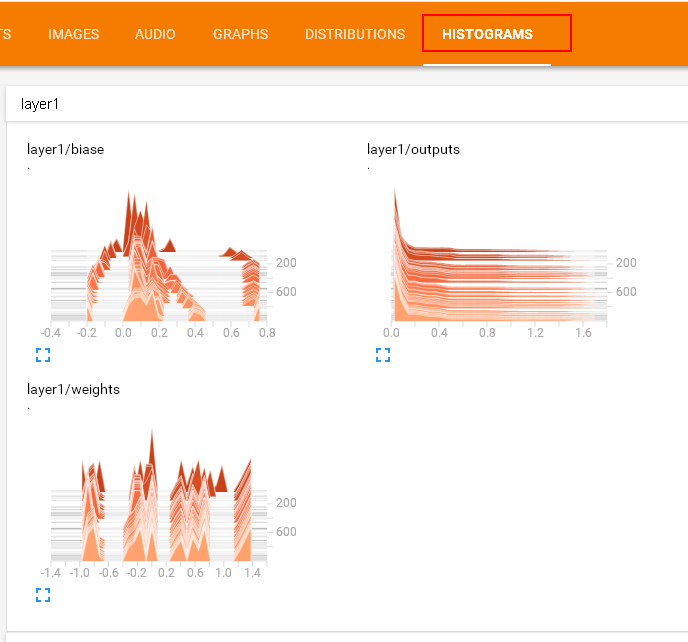
Histogram

使用summary histogram统计某个Tensor的取值分布:

 with tf.name_scope('layer1'):
          with tf.name_scope('biases'):
              biases = ... # 具体声明这里不再给出
              tf.summary.histogram('layer1' + '/biases', biases)

          with tf.name_scope('weights'):
              weights= ...
              tf.summary.histogram('layer1' + '/weights', weights)

          with tf.name_scope('outputs'):
              outputs= ...
              tf.summary.histogram('layer1' + '/weights', outputs)

合并Summary

# 将各个summary操作合并为一个操作merged_summary_op
merged_summary_op = tf.summary.merge_all()
# 数据写入器，'/logs'为训练日志的存储路径
summary_writer = tf.summary.FileWriter('./logs', sess.graph) 

total_step = 0
while training:
  total_step += 1
  session.run(training_op)
  if total_step % 100 == 0:
    ...
    summary_str = sess.run(merged_summary_op, feed_dict{...}) # 注意这里必须加feed_dict否则会报错
    summary_writer.add_summary(summary_str, total_step) # 使用summary_writer将数据写入磁盘

生成TensorBoard界面

运行添加了各种summary的操作的代码后，打开cmd，进入代码所在文件夹，输入：

tensorboard --logdir=logs

按照运行后的提示：

TensorBoard 1.7.0 at http://MengjieZhang:6006 (Press CTRL+C to quit)

打开浏览器，输入地址 http://MengjieZhang:6006 即可以看到TensorBoard界面。

具体代码：

input_data下载链接

import input_data
import tensorflow as tf

def weight_variable(shape):
  initial = tf.truncated_normal(shape, stddev=0.1)
  return tf.Variable(initial)

def bias_variable(shape):
  initial = tf.constant(0.1, shape=shape)
  return tf.Variable(initial)

def conv2d(x, W):
  return tf.nn.conv2d(x, W, strides=[1, 1, 1, 1], padding='SAME')

def max_pool_2x2(x):
  return tf.nn.max_pool(x, ksize=[1, 2, 2, 1],
                        strides=[1, 2, 2, 1], padding='SAME')

mnist = input_data.read_data_sets('data', one_hot=True)

mnistGraph = tf.Graph()
with mnistGraph.as_default():
    with tf.name_scope('input'):
        x = tf.placeholder("float", shape=[None, 784])
        y_ = tf.placeholder("float", shape=[None, 10])
        W = tf.Variable(tf.zeros([784,10]))
        b = tf.Variable(tf.zeros([10]))

    with tf.name_scope('hidden1'):
        W_conv1 = weight_variable([5, 5, 1, 32])
        b_conv1 = bias_variable([32])
        x_image = tf.reshape(x, [-1,28,28,1])
        h_conv1 = tf.nn.relu(conv2d(x_image, W_conv1) + b_conv1)
        h_pool1 = max_pool_2x2(h_conv1)
        tf.summary.histogram('W_conv1', W_conv1)
        tf.summary.histogram('b_conv1', b_conv1)

    with tf.name_scope('hidden2'):
        W_conv2 = weight_variable([5, 5, 32, 64])
        b_conv2 = bias_variable([64])
        h_conv2 = tf.nn.relu(conv2d(h_pool1, W_conv2) + b_conv2)
        h_pool2 = max_pool_2x2(h_conv2)
        tf.summary.histogram('W_conv2', W_conv2)
        tf.summary.histogram('b_conv2', b_conv2)

    with tf.name_scope('fc1'):
        W_fc1 = weight_variable([7 * 7 * 64, 1024])
        b_fc1 = bias_variable([1024])
        h_pool2_flat = tf.reshape(h_pool2, [-1, 7*7*64])
        h_fc1 = tf.nn.relu(tf.matmul(h_pool2_flat, W_fc1) + b_fc1)
        keep_prob = tf.placeholder("float")
        h_fc1_drop = tf.nn.dropout(h_fc1, keep_prob)
        tf.summary.histogram('W_fc1', W_fc1)
        tf.summary.histogram('b_fc1', b_fc1)

    with tf.name_scope('fc2'):
        W_fc2 = weight_variable([1024, 10])
        b_fc2 = bias_variable([10])
        y_conv=tf.nn.softmax(tf.matmul(h_fc1_drop, W_fc2) + b_fc2)
        tf.summary.histogram('W_fc2', W_fc2)
        tf.summary.histogram('b_fc2', b_fc2)

    with tf.name_scope('train'):
        cross_entropy = -tf.reduce_sum(y_*tf.log(y_conv))
        train_step = tf.train.AdamOptimizer(1e-4).minimize(cross_entropy)
        correct_prediction = tf.equal(tf.argmax(y_conv,1), tf.argmax(y_,1))
        accuracy = tf.reduce_mean(tf.cast(correct_prediction, "float"))
        tf.summary.scalar('loss', cross_entropy)
        tf.summary.scalar('accuracy', accuracy)      

with tf.Session(graph=mnistGraph) as sess:
    sess.run(tf.initialize_all_variables())
    merged_summary_op = tf.summary.merge_all()
    summary_writer = tf.summary.FileWriter('./logs', sess.graph)
    for i in range(3000):
      batch = mnist.train.next_batch(50)
      if i%100 == 0:
        train_accuracy = accuracy.eval(feed_dict={
            x:batch[0], y_: batch[1], keep_prob: 1.0})
        print ("step %d, training accuracy %g" % (i, train_accuracy))
        summary_str = sess.run(merged_summary_op, feed_dict={x: batch[0], y_: batch[1], keep_prob: 0.5})
        summary_writer.add_summary(summary_str, i)
      train_step.run(feed_dict={x: batch[0], y_: batch[1], keep_prob: 0.5})

    accuracy_sum = tf.reduce_sum(tf.cast(correct_prediction, tf.float32))
    good = 0
    total = 0
    for i in range(10):
        testSet = mnist.test.next_batch(50)
        good += accuracy_sum.eval(feed_dict={ x: testSet[0], y_: testSet[1], keep_prob: 1.0})
        total += testSet[0].shape[0]
    print ("test accuracy %g"%(good/total))

运行后的TensorBoard界面：