GoodReads: Machine Learning (Part 3)

In the first installment of this series, we scraped reviews from Goodreads. In thesecond one, we performed exploratory data analysis and created new variables. We are now ready for the “main dish”: machine learning!

Setup and general data prep

Let’s start by loading the libraries and our dataset.

library(data.table)
library(dplyr)
library(caret)
library(RTextTools)
library(xgboost)
library(ROCR)

setwd("C:/Users/Florent/Desktop/Data_analysis_applications/GoodReads_TextMining")
data <- read.csv("GoodReadsCleanData.csv", stringsAsFactors = FALSE)

To recap, at this point, we have the following features in our dataset:

review.id
book
rating
review
review.length
mean.sentiment
median.sentiment
count.afinn.positive
count.afinn.negative
count.bing.negative
count.bing.positive

For this example, we’ll simplify the analysis by collapsing the 1 to 5 stars rating into a binary variable: whether the book was rated a “good read” (4 or 5 stars) or not (1 to 3 stars). This will allow us to use classification algorithms, and to have less unbalanced categories.

set.seed(1234)
# Creating the outcome value
data$good.read <- 0
data$good.read[data$rating == 4 | data$rating == 5] <- 1

The “good reads”, or positive reviews, represent about 85% of the dataset, and the “bad reads”, or negative reviews, with good.read == 0, about 15%. We then create the train and test subsets. The dataset is still fairly unbalanced, so we don’t just randomly assign data points to the train and test datasets; we make sure to preserve the percentage of good reads in each subset by using the caret function `createDataPartition` for stratified sampling.

trainIdx <- createDataPartition(data$good.read,
                                p = .75,
                                list = FALSE,
                                times = 1)
train <- data[trainIdx, ]
test <- data[-trainIdx, ]

Creating the Document-Term Matrices (DTM)

Our goal is to use the frequency of individual words in the reviews as features in our machine learning algorithms. In order to do that, we need to start by counting the number of occurrence of each word in each review. Fortunately, there are tools to do just that, that will return a convenient “Document-Term Matrix”, with the reviews in rows and the words in columns; each entry in the matrix indicates the number of occurrences of that particular word in that particular review.

A typical DTM would look like this:

Reviews	about	across	ado	adult
Review 1	0	2	1	0
Review 2	1	0	0	1

We don’t want to catch every single word that appears in at least one review, because very rare words will increase the size of the DTM while having little predictive power. So we’ll only keep in our DTM words that appear in at least a certain percentage of all reviews, say 1%. This is controlled by the “sparsity” parameter in the following code, with sparsity = 1-0.01 = 0.99.

There is a challenge though. The premise of our analysis is that some words appear in negative reviews and not in positive reviews, and reversely (or at least with a different frequency). But if we only keep words that appear in 1% of our overall training dataset, because negative reviews represent only 15% of our dataset, we are effectively requiring that a negative word appears in 1%/15% = 6.67% of the negative reviews; this is too high a threshold and won’t do.

The solution is to create two different DTM for our training dataset, one for positive reviews and one for negative reviews, and then to merge them together. This way, the effective threshold for negative words is to appear in only 1% of the negative reviews.

# Creating a DTM for the negative reviews
sparsity <- .99
bad.dtm <- create_matrix(train$review[train$good.read == 0],
                         language = "english",
                         removeStopwords = FALSE,
                         removeNumbers = TRUE,
                         stemWords = FALSE,
                         removeSparseTerms = sparsity)
#Converting the DTM in a data frame
bad.dtm.df <- as.data.frame(as.matrix(bad.dtm),
                            row.names = train$review.id[train$good.read == 0])

# Creating a DTM for the positive reviews
good.dtm <- create_matrix(train$review[train$good.read == 1],
                          language = "english",
                          removeStopwords = FALSE,
                          removeNumbers = TRUE,
                          stemWords = FALSE,
                          removeSparseTerms = sparsity) 

good.dtm.df <- data.table(as.matrix(good.dtm),
                          row.names = train$review.id[train$good.read == 1])

# Joining the two DTM together
train.dtm.df <- bind_rows(bad.dtm.df, good.dtm.df)
train.dtm.df$review.id <- c(train$review.id[train$good.read == 0],
                            train$review.id[train$good.read == 1])
train.dtm.df <- arrange(train.dtm.df, review.id)
train.dtm.df$good.read <- train$good.read

We also want to use in our analyses our aggregate variables (review length, mean and median sentiment, count of positive and negative words according to the two lexicons), so we join the DTM to the train dataset, by review id. We also convert all NA values in our data frames to 0 (these NA have been generated where words were absent of reviews, so that’s the correct of dealing with them here; but kids, don’t convert NA to 0 at home without thinking about it first).

train.dtm.df <- train %>%
  select(-c(book, rating, review, good.read)) %>%
  inner_join(train.dtm.df, by = "review.id") %>%
  select(-review.id)

train.dtm.df[is.na(train.dtm.df)] <- 0

# Creating the test DTM
test.dtm <- create_matrix(test$review,
                          language = "english",
                          removeStopwords = FALSE,
                          removeNumbers = TRUE,
                          stemWords = FALSE,
                          removeSparseTerms = sparsity)
test.dtm.df <- data.table(as.matrix(test.dtm))
test.dtm.df$review.id <- test$review.id
test.dtm.df$good.read <- test$good.read

test.dtm.df <- test %>%
  select(-c(book, rating, review, good.read)) %>%
  inner_join(test.dtm.df, by = "review.id") %>%
  select(-review.id)

A challenge here is to ensure that the test DTM has the same columns as the train dataset. Obviously, some words may appear in the test dataset while being absent of the train dataset, but there’s nothing we can do about them as our algorithms won’t have anything to say about them. The trick we’re going to use relies on the flexibility of the data.tables: when you join by rows two data.tables with different columns, the resulting data.table automatically has all the columns of the two initial data.tables, with the missing values set as NA. So we are going to add a row of our training data.table to our test data.table and immediately remove it after the missing columns will have been created; then we’ll keep only the columns which appear in the training dataset (i.e. discard all columns which appear only in the test dataset).

test.dtm.df <- head(bind_rows(test.dtm.df, train.dtm.df[1, ]), -1)
test.dtm.df <- test.dtm.df %>%
  select(one_of(colnames(train.dtm.df)))
test.dtm.df[is.na(test.dtm.df)] <- 0

With this, we have our training and test datasets and we can start crunching numbers!

Machine Learning

We’ll be using XGboost here, as it yields the best results (I tried Random Forests and Support Vector Machines too, but the resulting accuracy is too instable with these to be reliable).

We start by calculating our baseline accuracy, what would get by always predicting the most frequent category, and then we calibrate our model.

baseline.acc <- sum(test$good.read == "1") / nrow(test)

XGB.train <- as.matrix(select(train.dtm.df, -good.read),
                       dimnames = dimnames(train.dtm.df))
XGB.test <- as.matrix(select(test.dtm.df, -good.read),
                      dimnames=dimnames(test.dtm.df))
XGB.model <- xgboost(data = XGB.train,
                     label = train.dtm.df$good.read,
                     nrounds = 400,
                     objective = "binary:logistic")

XGB.predict <- predict(XGB.model, XGB.test)

XGB.results <- data.frame(good.read = test$good.read,
                          pred = XGB.predict)

The XGBoost algorithm yields a probabilist prediction, so we need to determine a threshold over which we’ll classify a review as good. In order to do that, we’ll plot the ROC (Receiver Operating Characteristic) curve for the true negative rate against the false negative rate.

ROCR.pred <- prediction(XGB.results$pred, XGB.results$good.read)
ROCR.perf <- performance(ROCR.pred, 'tnr','fnr')
plot(ROCR.perf, colorize = TRUE)

Things are looking pretty good. It seems that by using a threshold of about 0.8 (where the curve becomes red), we can correctly classify more than 50% of the negative reviews (the true negative rate) while misclassifying as negative reviews less than 10% of the positive reviews (the false negative rate).

XGB.table <- table(true = XGB.results$good.read,
                   pred = as.integer(XGB.results$pred >= 0.80))
XGB.table
XGB.acc <- sum(diag(XGB.table)) / nrow(test)

Our overall accuracy is 87%, so we beat the benchmark of always predicting that a review is positive (which would yield a 83.4% accuracy here, to be precise), while catching 61.5% of the negative reviews. Not bad for a “black box” algorithm, without any parameter optimization or feature engineering!

Directions for further analyses

If we wanted to go deeper in the analysis, a good starting point would be to look at the relative importance of features in the XGBoost algorithm:

### Feature analysis with XGBoost
names <- colnames(test.dtm.df)
importance.matrix <- xgb.importance(names, model = XGB.model)
xgb.plot.importance(importance.matrix[1:20, ])

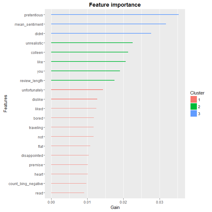
As we can see, there are a few words, such as “colleen” or “you” that are unlikely to be useful in a more general setting, but overall, we find that the most predictive words are negative ones, which was to be expected. We also see that two of our aggregate variables, review.length and count.bing.negative, made the top 10.

There are several ways we could improve on the analysis at this point, such as:

• using N-grams (i.e. sequences of words, such as “did not like”) in addition to single words, to better qualify negative terms. “was very disappointed” would obviously have a different impact compared to “was not disappointed”, even though on a word-by-word basis they could not be distinguished.
• fine-tuning the parameters of the XGBoost algorithm.
• looking at the negative reviews that have been misclassified, in order to determine what features to add to the analysis.

Conclusion

We have covered a lot of ground in this series: from webscraping to sentiment analysis to predictive analytics with machine learning. The main conclusion I would draw from this exercise is that we now have at our disposal a large number of powerful tools that can be used “off-the-shelf” to build fairly quickly a complete and meaningful analytical pipeline.

As for the first two installments, the complete R code for this part is available onmy github.

转自：https://www.r-bloggers.com/goodreads-machine-learning-part-3/